7  Functions and Multiple Regression

7.1 Functions in R

As was explained earlier, functions are the basic building blocks in R to get things done. John M. Chambers, the creator of the S programming language [1], and core member of the R programming language, once said:

• “Everything that exists, is an object.” and,
• “Everything that happens, is a function call.”.

R has many, many built-in functions. In this lesson you are going to look at R functions more carefully. Not only will you see how existing functions can be called, but also how easy it is to make your own! Actually, this is what people do if they make new packages: they program a new set of functions and spread them worldwide in an R package.

7.1.1 Exercise SWIRL: Functions

First you are going to use the swirl package to study functions.

Start up SWIRL by loading the package and starting it:

library(swirl)
swirl()

Choose the R Programming course, followed by Lesson 9: Functions.

WarningWarning: Answers in SWIRL

Keep in mind that answers in SWIRL Lessons are sensitive to the smallest of errors, so follow the instructions given in a lesson carefully!

In this lesson you will see:

• structure of a function: name, arguments between round brackets, body between curly brackets
• typing the name of function without brackets shows the source code
• last expression evaluated is returned by function
• default arguments for functions so that some arguments need not be specified in call
• function calls with explicitly names arguments, so that order is unimportant
• abbreviating names of arguments
• function args() to see arguments of a function
• functions as arguments to other functions
• anonymous functions
• ellipses \(\ldots\) argument for an indefinite number of arguments
• defining binary operators like +, -, *, /

7.1.2 Function Control Structure: The return() Function

In SWIRL Lesson 9 about Functions, you have just worked through, you have learned that the last expression evaluated in a function gets returned by the function. There is, however, also a control structure available, that will give you more control on what, and where objects get returned inside a function.

The return() function is used inside a new function definition and signals that a function should exit and return a given value.

An example of the use of return() inside a function definition and its use:

check <- function(x) {
  if (x > 0) {
    result <- "Positive"
  } else if (x < 0) {
    result <- "Negative"
  } else {
    result <- "Zero"
  }
  return(result)
}
# some sample runs.
check(1)

#> [1] "Positive"

check(-10)

#> [1] "Negative"

check(0)

#> [1] "Zero"

If there are no explicit returns from a function, as you have seen in the SWIRL Lesson 9, the value of the last evaluated expression is returned automatically in R.

For example, the following is equivalent to the above function:

check <- function(x) {
  if (x > 0) {
    result <- "Positive"
  } else if (x < 0) {
    result <- "Negative"
  } else {
    result <- "Zero"
  }
  result
}

Generally explicit use of the return() function to return a value immediately within a new function definition is advised. Mainly for readability of your code.

If return() is not the last statement of the new function definition, it will prematurely end the function bringing the control to the place from which it was called. For example:

check <- function(x) {
  if (x > 0) {
    return("Positive")
  } else if (x < 0) {
    return("Negative")
  } else {
    return("Zero")
  }
}

In the above example, if x > 0, the function immediately returns “Positive” without evaluating rest of the body.

The return() function can return only a single object. If you want to return multiple values in R, you need to use a list (or other objects) and return it.

Following is an example:

multi_return <- function() {
  my_list <- list("color" = "red",
                  "size" = 20,
                  "shape" = "round")
  return(my_list)
}
a <- multi_return()
a$color

#> [1] "red"

a$size

#> [1] 20

a$shape

#> [1] "round"

Here a list is created, named my_list inside the function multi_return(), with multiple elements and this single list is returned by the function named multi_return() and assigned to an object named a.

7.1.3 Example function: Standard Error of the Mean (s.e.m.)

As an example we make a function to calculate the standard error of the mean. This function is not available within basic R.

Suppose we have a random sample \(y_1,\ldots,\ y_n\) from some population with population mean \(\mu\) and standard deviation \(\sigma\). As estimator of \(\mu\) we use the sample mean \(\bar{y}\). As estimator of \(\sigma\) we take the sample standard deviation \(s\), available in R with function sd().

For hypothesis testing or confidence intervals for \(\mu\) we need (an estimator of) the standard error of the mean: \(sem = s / \sqrt{n}\). Below a function sem() is defined. It takes as argument a numerical vector \(y\) and returns the \(sem(y)\). Try the code yourself in R.

sem <- function(y) {
  n <- length(y)
  result <- sd(y) / sqrt(n)
  return(result)
}

Apply this function to some data. We sample 25 values from a standard normal distribution (\(\mu=0\), \(\sigma=1\)). The standard error of the mean should approximately be around \(1/\sqrt{25}=0.2\). Is this what you see below?

set.seed(seed = 1492) # ensure same pseudo random numbers for everyone
z <- rnorm(n = 25) # draw 25 numbers from N(0, 1)
mean(z) # calculate the mean

#> [1] -0.2579794

sd(z) # calculate the standard deviation

#> [1] 0.9903985

length(z) # number of observations in vector z

#> [1] 25

sem(z) # calculate the standard error of the mean

#> [1] 0.1980797

When random numbers are drawn with a computer, then these numbers are not complete random for they depend on the initialization (so-called pseudo random numbers). To ensure that always the same random numbers are drawn you can fix the initialization with the set.seed() function in R.

7.1.4 Exercise: Functions, Doing It Yourself (DIY)

Make an R function that takes three arguments:

1. a vector with numeric data to be summarized (possibly containing missing values)
2. a number of decimals to be printed; the default number should be 2
3. a logical telling whether missing values should be removed prior to calculating means and standard deviations; the default value should be TRUE.

The function should return a string, containing the mean and standard deviation in the form mean (standard deviation), like \(10.21~(2.13)\). [Hint: the function round() can be used to get the desired number of decimals; the function paste() can be used to create the desired string.]

7.2 Multiple regression

For theory see O&L Sections 12.1, 12.2, 12.3, 12.4, 12.5, 12.6, \(7^{\mbox{th}}\) Edition [2] Sections 13.2 pp.718-719, 13.4 p.745 and p.753 (\(6^{\mbox{th}}\) Edition [3]: Sections 13.2 pp.770-771, 13.4 p.797 and p.805).

The multiple linear regression model describes a linear relationship between dependent variable \(y\) and multiple regressors (explanatory variables) \(x_1, \ldots, x_k\): \[ y_i = \beta_0 + \beta_1 x_{1i} + \ldots + \beta_k x_{ki} + \varepsilon_i \tag{7.1}\]

with \(i=1, \ldots, n\) as an index for the observation number. As in simple linear regression, we assume that the errors \(\varepsilon_i\) are independent, have constant variance and are normally distributed with expected value 0.

Least-squares estimates of the parameters \(\beta_0\), \(\beta_1,\ \ldots,\ \beta_k\) are obtained using the R function lm(), like we did in simple linear regression. This function wants a model formula y ~ x1 + ... + xk as input. The results from the linear regression are saved into an R object of class lm. All functions shown in Lesson 4 on Simple Linear Regression can be used for multiple regression again.

Below we look at an example about yield of an orchard (\(y\)) and its possible dependency upon the average January (\(x_1\)) and May (\(x_2\)) temperatures. Observations have been collected during six consecutive years. The following multiple linear regression model is assumed: \(y_i = \beta_0 + \beta_1 x_{1i} + \beta_2 x_{2i} + \epsilon_i\) with \(i = 1 \ldots 6\).

Please type the commands shown below into an R script, or, even better, into an Rmd file.

y  <- c(31.4, 32.0, 32.3, 33.2, 32.7, 33.4)
x1 <- c( 0.5,  1.0,  2.0,  2.5,  3.0,  3.0)
x2 <- c(12.0, 12.0, 13.0, 14.0, 13.0, 14.0)

lmo <- lm(y ~ x1 + x2) # fit the multiple regression model
summary(object = lmo)  # summary of results

#> 
#> Call:
#> lm(formula = y ~ x1 + x2)
#> 
#> Residuals:
#>        1        2        3        4        5        6 
#> -0.16667  0.30000 -0.20000  0.03333 -0.06667  0.10000 
#> 
#> Coefficients:
#>             Estimate Std. Error t value Pr(>|t|)
#> (Intercept)  25.0333     2.6667   9.387  0.00256
#> x1            0.2667     0.1963   1.359  0.26737
#> x2            0.5333     0.2301   2.317  0.10332
#> 
#> Residual standard error: 0.2404 on 3 degrees of freedom
#> Multiple R-squared:  0.939,  Adjusted R-squared:  0.8983 
#> F-statistic: 23.08 on 2 and 3 DF,  p-value: 0.01508

confint(object = lmo)  # confidence intervals for parameters

#>                  2.5 %     97.5 %
#> (Intercept) 16.5465889 33.5200778
#> x1          -0.3579245  0.8912579
#> x2          -0.1990648  1.2657315

The \(F\)-test shown at the bottom of the output from summary() is the, so-called, “omnibus” \(F\)-test. It tests \(\mbox{H}_0:\ \beta_1 = \beta_2 = 0\). In words, it tests whether there is any explanatory power at all for this regression model.

We continue with some assumption checking, as shown in Figure 7.1. Notice the function rstandard() to obtain standardized residuals.

r <- residuals(object = lmo) # ordinary residuals
sr <- rstandard(model = lmo) # standardized residuals
f <- fitted(object = lmo)    # fitted values

# normal Q-Q plot using the standardized residuals
qqnorm(sr); qqline(sr, col = "red")

# residual plot; too few points to say anything about model assumptions:
plot(r ~ f,
     main = "Check constant variance",
     ylab = "residuals",
     xlab = "fitted values")
# add horizontal line residuals = 0 in residual plot
abline(h = 0)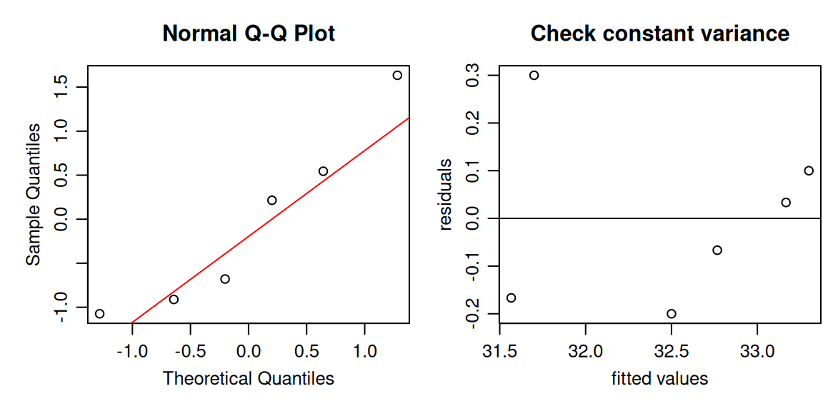

Figure 7.1: Plots to check the assumptions for multiple linear regression

We conclude with estimation of the mean response at new values of the regressors, including a confidence interval. Here we want to estimate the mean yield if the January temperature is 1°C and May temperature is 14°C.

newdata <- data.frame(x1 = 1, x2 = 14)
predict(object = lmo,
        newdata = newdata,
        se.fit = TRUE,
        interval = "confidence")

#> $fit
#>        fit      lwr     upr
#> 1 32.76667 31.42343 34.1099
#> 
#> $se.fit
#> [1] 0.422076
#> 
#> $df
#> [1] 3
#> 
#> $residual.scale
#> [1] 0.2403701

In simple linear regression we did not discuss the ANOVA table. The ANOVA table is a table, that tells how well the regression model is fitting, by comparing the multiple linear regression model with the simplest model possible, i.e. the model with only a constant (intercept). The residual sums of squares of these two models (which are the products of the least-squares procedure) are put in a table, together with the difference between the two. This difference (the model sum of squares) tells how much of the variation is explained by the regressors.

In R a “sort of” ANOVA table is obtained using the function anova(). First we are going to look at this function. Later we are going to modify it by creating a new function newAnova(), using the knowledge you gained in the previous Section 7.1.

anova(object = lmo)

#> Analysis of Variance Table
#> 
#> Response: y
#>           Df  Sum Sq Mean Sq F value   Pr(>F)
#> x1         1 2.35636 2.35636 40.7832 0.007775
#> x2         1 0.31030 0.31030  5.3706 0.103324
#> Residuals  3 0.17333 0.05778

The call anova(object = lmo) produces an “Analysis of Variance Table”, a.k.a ANOVA table. In the column Sum Sq sums of squares are shown.

At the bottom of the ANOVA table the residual sum of squares is presented, which is the result from the least-squares procedure. This is the value that can be obtained with the deviance() function.

deviance(object = lmo)

#> [1] 0.1733333

Further up in the table you see the contribution of each regressor to the model sum of squares. These are so-called sequential sums of squares, obtained by fitting a sequence of models. Let’s try to reproduce them, so that you understand how they are constructed.

Start with a model with only an intercept, and store the residual sum of squares of this model. Notice that we have to supply 1 as the right-hand-side of the model formula, to tell to R that we want a model with intercept only.

M0 <- lm(y ~ 1)
(SSE0 <- deviance(object = M0))

#> [1] 2.84

Next fit a model with intercept and \(x_1\), and store the residual sum of squares of this second model. Notice that specification of the explicit intercept (1) is not needed anymore (although it doesn’t harm if you would add it):

M1 <- lm(y ~ x1)
(SSE1 <- deviance(object = M1))

#> [1] 0.4836364

Calculate the difference in SSE0 and SSE1. Notice that this is exactly the sum of squares for \(x_1\) shown in the ANOVA table earlier.

(SS1x1 <- SSE0 - SSE1)

#> [1] 2.356364

Next add \(x_2\) to the model that already contains intercept and \(x_1\), and calculate again the difference in residual sums of squares. This is the sum of squares for \(x_2\) after \(x_1\), as shown in the earlier ANOVA table.

M2 <- lm(y ~ x1 + x2)
(SSE2 <- deviance(object = M2))

#> [1] 0.1733333

(SS1x2x1 <- SSE1 - SSE2)

#> [1] 0.310303

If we would change the order of terms, we will get a different ANOVA table (!):

anova(object = lm(y ~ x2 + x1))

#> Analysis of Variance Table
#> 
#> Response: y
#>           Df  Sum Sq Mean Sq F value   Pr(>F)
#> x2         1 2.56000 2.56000 44.3077 0.006911
#> x1         1 0.10667 0.10667  1.8462 0.267367
#> Residuals  3 0.17333 0.05778

Hence, it is NOT possible to say which effect is caused by \(x_1\) and which effect is caused by \(x_2\). It is only possible to say what the effect of e.g. \(x_1\) is if we also specify which model it is part of!

The order-dependence of sums of squares is caused by correlation among the regressors. This is called multicollinearity. The collinearity of a regressor with all the other regressors can be measured with the Variance Inflation Factor (VIF). A value for VIF equal to 1 tells that there is no collinearity of the variable with all others. The function vif() can be found in the R package car.

suppressWarnings(library(car)) # suppresses a warning message being printed
vif(mod = M2)

#>       x1       x2 
#> 3.666667 3.666667

The anova() function can be used to compare two nested models, a Full Model \(FM\) and a (smaller) Reduced Model \(RM\) as described in O&L Section 12.5 of both the \(6^{\mbox{th}}\) Edition [3] (p. 691) and the \(7^{\mbox{th}}\) Edition [2] (p.652). It produces an \(F\)-test (for a subset of regression coefficients). Below we compare the Full Model M2 (\(FM\)), containing both \(x_1\) and \(x_2\) with the smaller Reduced Model M1 (\(RM\)), containing \(x_1\) alone. In other words, we are testing \(\mbox{H}_0:\ \beta_2 = 0\) versus \(\mbox{H}_{\mbox{a}}:\ \beta_2 \ne 0\). The test statistic \(F\) can be calculated with: \[ F = \frac{(SSE_{RM}-SSE_{FM}) / (df_{RM}-df_{FM})}{SSE_{FM}/df_{FM}} \tag{7.2}\]

where \(SSE\) represents the sum of squares residuals and \(df\) the degrees of freedom of, respectively, the full model (\(FM\)) and the reduced model (\(RM\)).

anova(M1, M2)

#> Analysis of Variance Table
#> 
#> Model 1: y ~ x1
#> Model 2: y ~ x1 + x2
#>   Res.Df     RSS Df Sum of Sq      F Pr(>F)
#> 1      4 0.48364                           
#> 2      3 0.17333  1    0.3103 5.3706 0.1033

7.2.1 Exercise Multiple Regression: Electricity and Gas Prices in USA

We look at a data set about yearly electricity use per household in each of the 50 states in the USA (around 1990). The aim was to find out how electricity use \(y\) is related to the price of electricity (\(x_1\)), per capita income (\(x_2\)) and gas price (\(x_3\)). We assume a multiple linear regression model: \(y = \beta_0 + \beta_1 x_1 + \beta_2 x_2 + \beta_3 x_3 + \varepsilon\).

1. Read the data file into R.

2. Make a matrix scatterplot of the 4 variables (use pairs(), check ?pairs on how to use this function).

3. Fit a multiple linear regression model, explaining electricity use \(y\) from electricity price (\(x_1\)), per capita income (\(x_2\)) and gas price (\(x_3\)).

4. Test if the model has any explanatory value.

5. Give the estimated regression equation.

6. Give the estimate and standard error of \(\beta_3\) (the slope for price of gas).

7. Fit a simple linear regression model with \(x_3\) alone, and give the estimate and standard error of the slope of \(x_3\) now.

8. Compare the two values for slopes (from the multiple and simple regression models). What may be the reason for the difference?

9. Calculate the variance inflation factors for the three regressors.

7.2.2 Exercise Functions: Redefining the Regression ANOVA table

In this final, challenging, exercise for Lesson 7 you are going to program a new ANOVA function. Let’s call it newAnova(). It should modify the ANOVA table produced by the anova() function, in such a way that the new table has only three rows: one row for Model, one row for Residual, and one row for Corrected Total.

The columns of the new ANOVA table remain as they are.

The argument for the new function is an object of class lm, as produced by the lm() function.

The result of the new function is a numerical matrix with 3 rows and 5 columns. The column headings of the ANOVA table should be: Df, Sum Sq, Mean Sq, F value, Pr(>F). These are simply the column names, that can be assigned to the matrix with function colnames(). The row names of the ANOVA table should be: Model, Residuals, and Corr. Total. These are simply row names, that can be assigned to the matrix with function rownames().

Now program the new anova function named newAnova(). Within the body of the function do the following:

• Run the old anova() on the linear model object, and store the ANOVA table e.g. under object name oldm; force this result to become a matrix, using oldm <- as.matrix(oldm), so that the result is just a numerical matrix.
• Determine the number of rows \(nr\) of this matrix; this will be the number of regressors + 1.
• Create a new matrix with 3 rows and 5 columns.
• Assign the last row of this old matrix to the second row in the new matrix.
• In the old matrix, add degrees of freedom (column 1) and sums of squares (column 2) of row 1 up to (and including) row \(nr - 1\); you may use the function colSums() for this.
• These accumulated values are the model degrees of freedom and model sum of squares of the new matrix, so put them in the first row (columns 1 and 2) of the new matrix.
• Based upon the degrees of freedom and sum of squares, calculate the mean square, the \(F\)-statistic, and the \(P\)-value (using the pf() function), and enter these numbers in columns 3, 4, and 5 of the first row of the new matrix.
• Fit the intercept-only model, so model formula y ~ 1 ; for this we need the dependent variable \(y\) itself; you can get it out of the linear model object with the extractor function model.frame() (assuming that the linear model object has name lmo): y <- model.frame(lmo)[, 1].
• Run the old anova() on the intercept-only result and force the result to be a matrix (which has only one row).
• Copy this row into row 3 of the new matrix.
• Add proper column names and row names (see above).
• Print the resulting new matrix

The result for the old and new anova functions, applied to the regression for the orchard data, should look like this:

anova(lmo)

#> Analysis of Variance Table
#> 
#> Response: y
#>           Df  Sum Sq Mean Sq F value   Pr(>F)
#> x1         1 2.35636 2.35636 40.7832 0.007775
#> x2         1 0.31030 0.31030  5.3706 0.103324
#> Residuals  3 0.17333 0.05778

newAnova(lmo)

#>             Df    Sum Sq    Mean Sq  F value     Pr(>F)
#> Model        2 2.6666667 1.33333333 23.07692 0.01507807
#> Residuals    3 0.1733333 0.05777778       NA         NA
#> Corr. Total  5 2.8400000 0.56800000       NA         NA

7.3 Command Reference

Lesson 7 commands

Command	Description
\(\ldots\)	ellipses argument in function definition, see ?dots for help
function()	define new functions in the R language
model.frame()	extract the model frame from a formula or fit
pairs()	produce a matrix of scatterplots
pf()	distribution function for the \(F\)(\(df_{num}\), \(df_{denom}\)) distribution
return()	explicitly output the object, given as argument, in a function
rstandard()	provide standardized residuals of a fitted model object \%
set.seed()	initialize the start for random number generation
suppressWarnings()	evaluate ignoring all warnings
vif()	calculate variance inflation factors for (generalized) linear models

[1]

J.M. Chambers, Programming with data: A guide to the S language, Springer Science & Business Media, 1998.

[2]

R.L. Ott, M. Longnecker, An introduction to statistical methods & data analysis, \(7^{\mbox{th}}\) Edition, Cengage Learning, 20 Channel Center Street, Boston, MA 0210, USA, 2016.

[3]

R.L. Ott, M. Longnecker, An introduction to statistical methods and data analysis, \(6^{\mbox{th}}\) International Student Edition, Brooks/Cole, Cengage Learning, 2010.